H3: Uber's open source hierarchical hexagonal grid for the world
The geospatial community is contemplating the pro's and con's of Uber's H3 discrete global grid system. The quick facts:
- A global geospatial indexing system, i.e. multi-precision tiling of the world with hierarchical linear indexes to organize data
- 16 resolutions
- The grid approximates geo features such as polygons or points, avoiding expensive geospatial operations --> exhibits great scaling behavior
-
It's a discrete global grid system, i.e. it breaks up the world into discrete cells, where every position in the world has a cell identifier associated with it
-
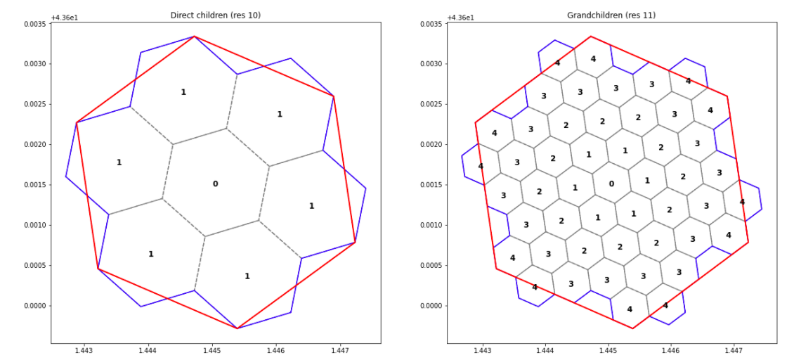
H3 is a system of grids. All 16 grid resolutions of the grid relate to each other; the resolution 10 grid is created by subdividing the resolution 9 grid and so forth
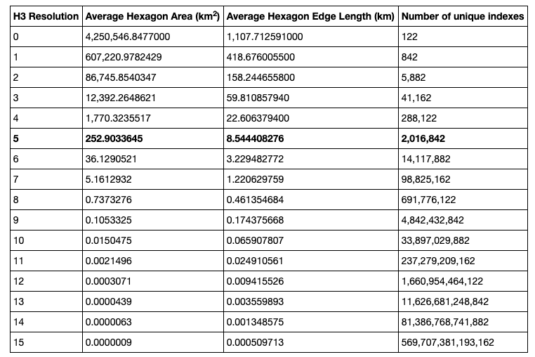
- This table show the different spatial dimensions per resolution (0-15 is 1-16)
Nice
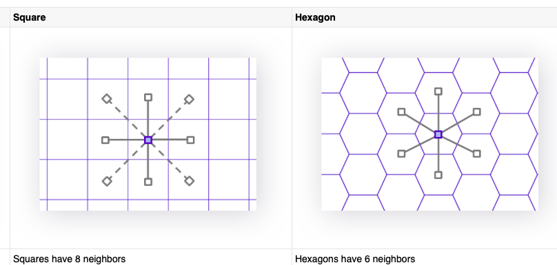
- A hexagonal system is more convenient for modeling spatial transformations, because neighbors are equal distant
- Uniform adjency neat property: all neighbors are the same distance apart
- When using H3, a point, a polygon, or any kind of shape gets coordinates, plus a resolution, and an indexing operation. The indexing operation is exactly at that resolution. The result is a list of indexes/identifiers for every single point of interest (e.g. building, market, hospital)
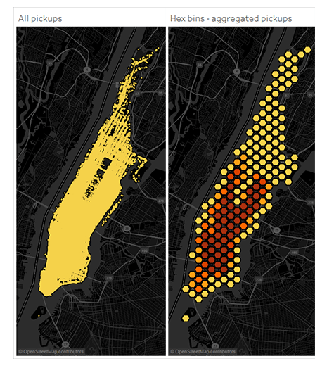
Usecase: Binning, database look-ups and categorisation
When working with large data sets, a great way to simplify the visual representation of complex point data is to spatially aggregate the points into bin regions so that you can look at groups of data instead of the individual points
-
You can map a data source from the H3 identifier to a metric value for that cell and do database lookups. For example, you can answer the question: "I'm in this area, I want to know how many buildings there are around me"
-
It’s just a matter of checking coordinates, finding the H3 identifier, and then looking that up in a database that is set up to map from the H3 identifier to that metric value
-
Great use case: binning and categorisations source
Binning mitigates variable resolution of source data and reduces computational complexity of feature engineering
-
When using a binning strategy to aggregate base points geographically, h3 is a great tool
- For example: H3 generates an H3 bin from a set of coordinates, and a boundrary shape for an H3 bin. In conjunction, these functions allow us to assign a bin to each point of interest, and then use that bin's geography to extract geodata from the raster datasets
-
With H3 all cells within a defined search distance can be looked up easily
-
-
It doesn't really know what you put next to it inside of your database. You could create a database in a Big Data system where one of those columns is an H3 identifier. The other columns can be whatever you want them to be, within the constraints of that database. You can attach categorical or numerical metrics to it
-
There are different ways to get a raster into the H3 grid. One is by sampling from the raster. We take an H3 grid, and we find some points we want to sample from the raster. Then we use that to move that raster data into the grid. Another way is by taking all the pixels in that raster and finding the associated H3 cell and moving the data in that way.
-
Unify data spatially
-
However, the hexagonal hierarchy could be a disadvantage when dividing hierarchies into smaller units. Spatial errors are not present, for instance, in squares
-
As a good example, in the US, we have customer data in zip code format, and we have demographics data in a format we'd get from the US Census Bureau. They use different geometries which the H3 grid joins together. We can also bring in raster, GPS tracks and all these different data and unify them into a simple analysis that the user is doing. It makes it a lot easier to access geospatial data.
Coversion in and out of H3
The ability to convert data back out of hexagons is just as critical. This allows you to transform between that sample of the US Census of geographies to zip codes. We're able to use a hexagon grid to transform remarkably efficiently from one polygon geometry to another. Users can do their analysis in a geometry that they're comfortable with and that they feel useful.
- Functions:
polyfillH3 polyfill takes an input polygon and finds the H3 indexes which cover it. So you can take a given input polygon that you re interested in and then find the index H3 grid that covers it. So you use the system from within a geometry rather than having to use the grid as the first instance of coverage.- Radius Lookup: You can use H3 for an efficient radius lookup, as long as you're willing to approximate the circle as a k-ring of hexagons (roughly, a large hexagonal shape). This is much faster than a true search by Haversine distance, but less accurate.
    h3_distance(H3Index origin, H3Index h3)
        Get the grid distance between H3 addresses.
        Returns the distance in grid cells between the two indexes.
        Returns a negative number if finding the distance failed.
        Finding the distance can fail because the two indexes are not comparable
        (different resolutions), too far apart, or are separated by pentagonal distortion.
        This is the same set of limitations as the local IJ coordinate space functions.
#haversine distance calc example:
    def haversine_dist(lon_src, lat_src, lon_dst, lat_dst):
        '''returns distance between GPS points, measured in meters'''
        lon1_rad, lat1_rad, lon2_rad, lat2_rad = map(np.radians,
                                                     [lon_src, lat_src, lon_dst, lat_dst])
        dlon = lon2_rad - lon1_rad
        dlat = lat2_rad - lat1_rad
        a = np.sin(dlat / 2.0) ** 2 + np.cos(lat1_rad) * \
            np.cos(lat2_rad) * np.sin(dlon / 2.0) ** 2
        c = 2 * np.arcsin(np.sqrt(a))
        km = 6367 * c
        return km * 1000
Fantastic notebook here
Check out this excellent podcast by mapscaping
Scaling Geospatial Workloads
- Usecase for friction modelling
- If we are handling shape files at large scale h3 might be useful