Download and analyse SARB BA900 forms

This is a description of the ba900 programm at https://github.com/t1nak/ba900/

Attention: requires python 2.7! Yes, the old one. I coded this up a long time ago. I will probably transcribe it to python 3 at some point. So long, you must create a python environment with python=2.7 because basestring is missing in python 3.

Other dependencies: lxml and more_itertools (pypi)

Get the South African Reserve Bank BA 900 forms

Time series of SA banks' balance sheets items

bubbles

top4 portfolio weights

top10 similarity full

I provide the data as of 24 October 2020 in this repo. If you want to update and download yourself, use the following steps.

Step 1

Run this snippet to create the folder data/downloaded in your project directory and one for each year available on the website:

import os
folder='data/downloaded'
path = os.path.join(os.getcwd(),folder)
years = [i for i in range(2008, 2021, 1)]

for y in years:
    if not os.path.exists(os.path.join(path,str(y))):
        os.makedirs(path+str(y))

Step 2

Download all the xml files from the SARB's homepage and unzip into the corresponding folder. If I find time I will add a little selenium function to do this automatically, but it's very simple as it is :)

Step 3

To convert the data from xml to dataframe run python ba900.py or the following snipped with the folder name you just created. The script will extract all data from the xml files and save as year.pkl

import pandas as pd 
from collections import Counter
from lxml import etree
import numpy as np
import os, sys
sys.path.insert(0,os.getcwd())
from extract_data import *
from iteration import *
import pickle

input = os.path.join(os.getcwd(), 'data/downloaded/')
output = os.path.join(os.getcwd(), 'data/output/')

if not os.path.exists(input): 
    os.mkdir(input)

if not os.path.exists(output): 
    os.mkdir(output)

years = [ 2008, 2009, 2010, 2011, 2012, 2013, 2014, 2015, 2016, 2017, 2018, 2019, 2020]

data = save_yearly_data(years, folder)

#This will save all years as one giant pickle (approx. 2GB)
#Uncomment if you want this
# filename =  os.path.join(folder, 'all_data.pickle')
# with open(filename, 'wb') as f:
#     pickle.dump(data, f)

print('All done. Have fun analysing.')nt('All done. Have fun analysing.')

After calling ba900.py you should see something like this:

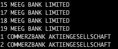
So the banks and their respective monthly data are being processed. It takes about 30 to 40 min to run all the bank and years (2008 to 2020).

Step 4

Now you have the data - great. However, analysis of the data requires good understanding of the ba900 forms. Here is a csv for ABSA, December 2008. - download link

There are 18 tables and 383 unique Item numbers. For example asset side positions are item numbers 103 to 277.

After familiarising yourself with the structure, you can load the pickled data and look at the time series with something like this

#load data
import os
import pandas as pd
import matplotlib.pyplot as plt
import numpy as np
import datetime
file_list=[]
for filename in os.listdir('./data/output/'):
    if filename.endswith(".pkl"):
        unpickle = './data/output/'+str(filename)
        print(unpickle)
        file_list.append(pd.read_pickle(unpickle))


MASTER = pd.concat(file_list)
MASTER['time'] = pd.to_datetime(MASTER['time'])

#print all column names
print(MASTER.columns)

Print all banks in the data set with print(MASTER['InstitutionDescription'].unique())

Look at ABSA bank asset portfolio weights:

#need assets_to_weights.py 
from assets_to_weights import *
transform=tranformer()

years=[str(i) for i in range(2008,2020, 1)]
months=["{:02d}".format(i) for i in range(1,13)]

helper_dict={}

for y in years:
    helper_dict[y]=months

BANK = MASTER[MASTER['InstitutionDescription']=='ABSA BANK LTD ']
BANK['Value'] = pd.to_numeric(BANK['Value'])

bank_year_and_month = []
for key in helper_dict.keys():
    for month in helper_dict[key]:

        df_bank_key_month =  BANK[(BANK['TheYear']==key)&(BANK['TheMonth']==month)]
#         print((month),(key),df_bank_key_month )
        try:
            bank_year_and_month.append(transform.get_pf_weights_by_bank_29(df_bank_key_month))
        except:
            pass

absa=pd.concat(bank_year_and_month) 

# we only need one entry per month - so select column code 7 and itemnumber 2 for example 
absa_weights=absa[(absa['ColumnCode']=='7')&(absa['ItemNumber']=='2')]
absa_weights.index=absa_weights.time

f = plt.figure()
plt.title('ABSA portfolio weights', color='black')

for column in absa_weights[absa.columns[-19:-10]]:
    absa_weights[column].plot(legend=column, ax=f.gca())
plt.legend(loc='center left', bbox_to_anchor=(1.0, 0.5))
plt.show()

absa portfolio weights

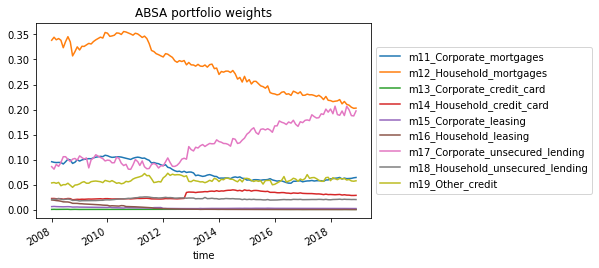
So you can see the gradual decline in household mortgage credit in ABSA's balance sheet as a share of its total balance sheet size.

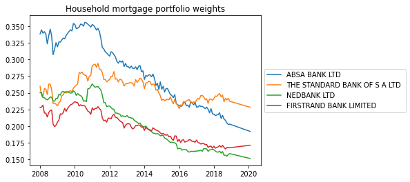
For the top 4 banks:

# show portfolio weights for absa's credit book
from assets_to_weights import *

transform=tranformer()

years=[str(i) for i in range(2008,2021, 1)]
months=["{:02d}".format(i) for i in range(1,13)]


top5=[ 'ABSA BANK LTD ',\
        'THE STANDARD BANK OF S A LTD ',\
        MASTER[MASTER['InstitutionDescription'].str.contains('NEDBANK')]['InstitutionDescription'].values[0],\
        MASTER[MASTER['InstitutionDescription'].str.contains('FIRSTRAND')]['InstitutionDescription'].values[0],\
        MASTER[MASTER['InstitutionDescription'].str.contains('CAPITEC BANK')]['InstitutionDescription'].values[0]
      ]

df=MASTER[MASTER.InstitutionDescription.isin(top5)]
arr = np.empty((0,len(df[df['InstitutionDescription'].str.contains('ABSA BANK LTD ')].time.unique()))) 

for b in top5:
    test=transform.get_bankdata(years,months,df, b)

    # # we only need one entry per month - so select column code 7 and itemnumber 2 for example 
    test_weights=test[(test['ColumnCode']=='7')&(test['ItemNumber']=='2')]
    test_weights.index=test_weights.time
    # f = plt.figure()
    # plt.title('ABSA portfolio weights', color='black') 
    # for column in test_weights[test.columns[-19:-10]]:
    #     test_weights[column].plot(legend=column, ax=f.gca())
    # plt.legend(loc='center left', bbox_to_anchor=(1.0, 0.5))
    # plt.show()
    weights_only=test_weights[test_weights.columns[-29:]] 
    d=weights_only.filter(like='Household_mortgages').squeeze().values 
    arr=np.vstack((arr,d))

import matplotlib.pyplot as plt

top5=[ 'ABSA BANK LTD ',\
        'THE STANDARD BANK OF S A LTD ',\
        MASTER[MASTER['InstitutionDescription'].str.contains('NEDBANK')]['InstitutionDescription'].values[0],\
        MASTER[MASTER['InstitutionDescription'].str.contains('FIRSTRAND')]['InstitutionDescription'].values[0],\
        MASTER[MASTER['InstitutionDescription'].str.contains('CAPITEC BANK')]['InstitutionDescription'].values[0]
      ]

f = plt.figure()
plt.title('Household mortgage portfolio weights', color='black')

for i,name in zip(arr[:-1],top5[:-1]):
    plt.plot(test_weights.time,i , label=name)

plt.legend(loc='center left', bbox_to_anchor=(1.0, 0.5))
plt.show()

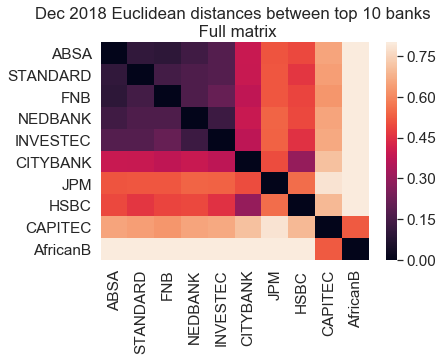
Euclidean distances betwenn top 10 banks (dec 2018):

top10 similarity half

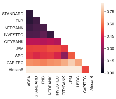
You can check some examples in the exame_analyse.ipynb notebook.

Write me if you have questions. There is a lot of scope to make this more user-friendly and if I get more feedback I will gladly do so. However, for my own purposes it has been sufficient like it is.